
Shortest Path Algorithm Comparison
This post will compare two of the popular algorithms used to attack this shortest-path problem in graph theory, Floyd’s algorithm and Dijkstra’s algorithm. I will briefly describe each algorithm, compare the two, and then provide guidelines for choosing between them. In addition, I will describe the results of test cases I ran on both algorithms.
The shortest path problem is the problem of finding a path between two vertices of a graph with a minimum total edge weight. The application of shortest path algorithms is useful in solving many real-world problems. They can be applied to network and telecommunications problems in order to find paths with the lowest delay. Additionally, mapping software utilized these types of algorithms to find the optimum route between two cities.
Both the Floyd’s algorithm and Dijkstra’s algorithm are examples of dynamic programming. Dynamic programming is a technique for solving problems by breaking them into smaller sub-problems. Each sub-problem is solved only once and the results are stored for later use. Dynamic programming algorithms are more resource intensive than their non-dynamic counterparts, which give them a higher space complexity. However, this higher space complexity should be offset with a lower time complexity. This time complexity reduction will often be linear, and while the theoretical gain is minimal, the actual performance increase may be significant.
Floyd’s Algorithm
Stephen Warshall and Robert Floyd independently discovered Floyd’s algorithm in 1962. In addition, Bernard Roy discovered this algorithm in 1959. This algorithm is sometimes referred to as the Warshall-Floyd algorithm or the Roy-Floyd algorithm. The algorithm solves a type of problem call the all-pairs shortest-path problem, meaning that it finds the shortest path between all the vertices of a given graph. Actually, the Warshall version of the algorithm finds the transitive closure of a graph but it does not use weights when finding a path. The Floyd algorithm is essentially the same as the Warshall algorithm except it adds weight to the distance calculation.
This algorithm works by estimating the shortest path between two vertices and further improving that estimate until it is optimum. Consider a graph G, with Vertices V numbered 1 to n. The algorithm first finds the shortest path from i to j, using only vertices 1 to k, where k<=n. Next, using the previous result the algorithm finds the shortest path from i to j, using vertices 1 to k+1. We continue using this method until k=n, at which time we have the shortest path between all vertices. This algorithm has a time complexity of O(n3), where n is the number of vertices in the graph. This is noteworthy because we must test up to n2 edge combinations.
Dijkstra’s Algorithm
Edsger Dijkstra discovered Dijkstra’s algorithm in 1959. This algorithm solves the single-source shortest-path problem by finding the shortest path between a given source vertex and all other vertices. This algorithm works by first finding the path with the lowest total weight between two vertices, j and k. It then uses the fact that a node r, in the path from j to k implies a minimal path from j to r. In the end, we will have the shortest path from a given vertex to all other vertices in the graph. Dijkstra’s algorithm belongs to a class of algorithms known as greedy algorithms. A greedy algorithm makes the decision that seems the most promising at a given time and then never reconsiders that decision.
The time complexity of Dijkstra’s algorithm is dependent upon the internal data structures used for implementing the queue and representing the graph. When using an adjacency list to represent the graph and an unordered array to implement the queue the time complexity is O(n2), where n is the number of vertices in the graph. However, using an adjacency list to represent the graph and a min-heap to represent the queue the time complexity can go as low as O(e*log n), where e is the number of edges. It is possible to get an even lower time complexity by using more complicated and memory intensive internal data structures, but that is beyond the scope of this paper.
Comparisons and Experiment
When using a naive implementation of Dijkstra’s algorithm the time complexity is quadratic, which is much better that the cubic time complexity of the Floyd’s algorithm. However, Dijkstra’s algorithm returns only a subset of Floyd’s algorithm. Specifically, it returns the shortest path between a given vertex and all other vertices while the Floyd’s algorithm returns the shortest path between all vertices. It is interesting to note that if you run Dijkstra’s algorithm n times, on n different vertices, you will have a theoretical time complexity of O(n* n2)=O(n3). In other words, if you use Dijkstra’s algorithm to find a path from every vertex to every other vertex you will have the same efficiency and result as using Floyd’s algorithm.
In order to test the efficiency of these algorithms I ran several test cases. I implemented Dijkstra’s algorithm using a priority queue and I ran each test case 1,000 times. All of the results are aggregations of the 1,000 runs, which gives me a larger, more manageable number. I ran six test cases, for each algorithm, varying the number of vertices in the graph. I used an automated method for creating edge so the sparseness of each graph is always the same.
In my implementation, the Floyd algorithm is actually faster when the number of vertices is small. Only after the number of vertices grows to more than ten does the Dijkstra algorithm become faster. When running Dijkstra’s algorithm n times (to get all-pairs shortest-path) the time complexity quickly grows greater that Floyd’s algorithm. Additional tests show that when running Dijkstra’s algorithm for more than a quarter of the vertices the time complexity exceeds that of Floyd’s algorithm.
The chart in figure 1 shows the total number of seconds for various values of n (for 1,000 iterations of each algorithm). As the number of vertices doubles from 80 to 160, the time increases by a factor 8, which is cubic time complexity. There is only a small increase in time complexity for Dijkstra’s algorithm over the same values for n. In fact, the time for Dijkstra’s algorithm increases by 2.3 as the value of n doubles, which is a logarithmic time complexity.

Figure 1
However, we must keep in mind that Floyd’s algorithm finds the shortest path between all vertices, while Dijkstra’s algorithm finds the shortest path from a single vertex to all other vertices. Therefore, the comparison between the two is not necessarily valid. If we want to use Dijkstra’s algorithm to find the shortest path for all vertices we must run it n times – once for each vertex.
The chart in figure 2 shows the total number of seconds for the same values of n, but with each iteration of Dijkstra’s algorithm being repeated n times. The result is that Dijkstra’s algorithm has also found the shortest path between all vertices but we the time requires increases by 6 when the value of n doubles.
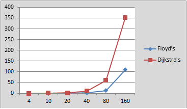
Figure2
In order to find the point at which Floyd’s algorithm is more efficient that Dijkstra’s algorithm I ran an addition test, only using the graphs with 80 nodes. The chart in figure 3 shows the results for finding the paths for a varying number of vertices. It shows that finding the shortest path for 21 vertices takes about 13 seconds, which is higher than the 12.65 seconds Floyd’s algorithm need to find all paths.

Figure3
Table 1 below gives the raw data used for the charts in figure 1 and 2. Table 2, shows the raw data for Dijkstra’s algorithm when called for a different number of vertices.

Conclusion
Both Floyd’s and Dijkstra’s algorithm may be used for finding the shortest path between vertices. The biggest difference is that Floyd’s algorithm finds the shortest path between all vertices and Dijkstra’s algorithm finds the shortest path between a single vertex and all other vertices. The space overhead for Dijkstra’s algorithm is considerably more than that for Floyd’s algorithm. In addition, Floyd’s algorithm is much easier to implement.
In most cases, for a small values number of vertices, the savings of using Dijkstra’s algorithm are negligible and probably not worth the effort and overhead required. However, when the number of vertices increases the performance of Floyd’s algorithm drops quickly. Therefore, the use of Dijkstra’s algorithm can provide a solution when performance is a factor. On the other hand, if you will need the shortest path between several vertices on the same graph you may want to consider Dijkstra’s algorithm. In the test case, running the algorithm for more than ¼ of the vertices decreased performance below that of running Floyd’s algorithm.